SequentialConvexRelaxation.jl

09 Sep 2019

I released the Julia package SequentialConvexRelaxation.jl, which applies a series of convex optimizations as a heuristic optimization method for nonconvex problems that can be described as convex problems with additional bilinear equality constraints. The software can be found here.

What does this package do?

This package (code) gives a convenient approach to attempt to solve nonconvex optimization problems that can be expressed as convex problems with additional bilinear equality constraints. The approach has worked well for me, and now I hope it will work well for you.

Bilinear equality constraints are constraints of the form $APB=C$ , where $A$ and $B$ are (matrix valued) decision variables, $P$ is a constant matrix and $C$ is either a decision variable or a constant matrix. The additional bilinear equality constraints make the overall optimization problem (in general) non-convex and non-linear. This package uses a convex heuristic approach to find good and feasible solutions at the same time.

It’s built on top of the package Convex.jl, but I am not affiliated with that project, nor are those authors with this project.

Why use it?

The advantages:

The ease of use of Convex.jl to model your optimization problem.
Only an SDP solver needed.
No initial feasible guess is necessary for the solver to start.
Only 1 regularization parameter to tune (if necessary) for every bilinear equality constraint.

The disadvantages:

No convergence guarantees (the problem is non-convex and non-linear after all). No guarantees of finding global optima, or feasible solutions.
High computational complexity of iterations.
Depending on the solver and the size and type of the problem, numerical issues in the solvers can spoil the fun.

Example problems with bilinear equality constraints

The Rosenbrock function

The Rosenbrock function is the nonconvex function

$f(x,y) = (a-x)^2 + b(y-x^2)^2$

where we use $a = 1,~ b = 100$ .

The problem of finding the minimum can be written as

$\begin{equation} \begin{aligned} & \text{minimize}_{x,y} && (a-x)^2 + b(y-x^2)^2 \end{aligned} \end{equation}$

Equivalently we might write

$\begin{equation} \begin{aligned} & \text{minimize}_{x,y,z} && (a-x)^2 + bz^2 \\ & \text{subject to} && x^2 = y-z \end{aligned} \end{equation}$

The objective function by itself is convex in $x$ and $z$ , and the constraint is a quadratic equality constraint (a subset of bilinear equality constraints). If there would be convex constraints on the variables, for example a linear inequality constraint like $x \geq -1$ , then we would group this with the convex problem.

Other examples

Other examples of problems that fit into this category that I can give here are:

Finding solutions for the travelling salesman problem
Training a neural network
Solving sudokus
Phase retrieval in optics
Blind deconvolution in optics
Structured robust optimal output feedback controller design
Several system identification (parameter estimation) problems.

I’m always interested in hearing about other examples, so if you have one (or if you’re not sure if you have one and would like some feedback), get in touch!

How to use it? A beginner’s tutorial.

Using this package requires five steps:

Construct the convex problem part using Convex.jl
Construct the bilinear equality constraints using BilinearConstraint()
Construct the BilinearProblem() using the two parts above
Give this to the solve!() function
Verify the results for feasibility in your original problem.

Let’s go over these steps for finding the minimum of the Rosenbrock function example above.

Installation

(v1.1) pkg> add https://github.com/rdoelman/SequentialConvexRelaxation.jl

Startup

using Convex
using SequentialConvexRelaxation
using SCS

a = 1.
b = 100.

# The Rosenbrock function
# f(x,y) = (a-x)^2 + b*(y-x^2)^2

x = Variable()
y = Variable()
z = Variable()

Step 1: Construct the convex problem part using Convex.jl

p = minimize(norm([a-x; sqrt(b)*z]))

Step 2: Construct the bilinear equality constraints

The function BilinearConstraint(A,P,B,C;X,Y,λ,W1,W2) specifies a bilinear equality constraint of the form $APB=C$ , with (optional) X some guess for -A, Y some guess for -B, λ a weighting parameter for weighting the regularization with the objective function, and W1 and W2 are internal weighting matrices (see below). I’m guessing -1 as an initial guess for $x_0$ and set the tuning parameter $\lambda$ to 0.1. You can play with these settings in the interactive example in the file “examples/rosenbrock.jl”.

x0 = -1
λ = 0.1
bc = BilinearConstraint(x,1.,x,y-z,X=-x0,Y=-x0,λ=λ)

Since constraints of the form $A \in \{0,1\}$ can be formulated as bilinear equality constraints, the function BinaryConstraint(A;X,W1,λ) provides a shortcut.

Step 3: Construct the `BilinearProblem()` using the two parts above

bp = BilinearProblem(p,bc)

If there is more than one bilinear equality constraint, supply a vector of BilinearConstraints.

Step 4: Give this to the `solve!()` function

An SDP (semidefinite programming) solver is needed to run the package’s solve! function (which calls Convex.jl’s solve!). SCS can be used. I found Mosek more numerically stable. I have no experience with other solvers.

r = solve!(bp,SCSSolver(verbose=0),iterations=2, trackvariables=(x,y))

The number of iterations can be supplied, but it defaults to 1. For this specific example with these settings, 2 is sufficient, but sometimes many more are necessary. Check out the rosenbrock.jl example file to get a feeling for how tuning works.

If you give a tuple of Convex.AbstractExpr (like Variables) these will be evaluated at every iteration and returned in the Result object r, along with some more information from the process. This Result object is also stored in the BilinearProblem bp.

Step 5: Verify the results for feasibility in your original problem.

As indicated before, the package applies a heuristic method that might or might not produce a feasible answer. It should be checked whether the bilinear equality constraints are satisfied. The solve! function produces a warning if the constraints are not satisfied within a small tolerance.

Note that solve! can modify values in the convex problem and the bilinear equality constraints, so calling it twice in a row might give unexpected results.

Depending on the problem and the solver I sometimes encounter numerical issues, where the bilinear equality is practically satisfied, but after substitution in the original problem, some constraints might be violated by a tiny amount. This matters in some applications, so it’s worth checking before proceeding with the results.

The result of the above code when plotted should look like this:

Rosenbrock minimization

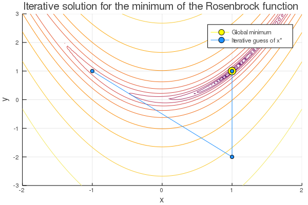
A side note with this figure is that the y-value of the blue dot on the left (the starting point) was set arbitrarily by me for plotting purposes, since there is no correct value.

Further documentation

Documentation can be found using ?functionname in the Julia REPL and over at the GitHub repository page.

How does the package mathematically work?

Given a problem of the form

$\begin{equation} \begin{aligned} & \text{minimize} && f \\ & \text{subject to} && A_iP_iB_i=C_i, \quad i = 1,\ldots,N \end{aligned} \end{equation}$

where $f$ is a convex function, and $A_iP_iB_i=C_i$ is a bilinear matrix-valued (or scalar-valued) equality constraint, the package iteratively solves

$\begin{equation} \begin{aligned} & \text{minimize} && f + \sum_{i=1}^N λ_i \| M_i \|_* \\ & \text{subject to} && M_i := \begin{bmatrix} W_{1,i} (C_i + A_iP_iY_i + X_iP_iB_i + X_iP_iY_i) W_{2,i} & W_{1,i}(A_i+X_i)P_i \\ P_i(B_i+Y_i)W_{2,i} & P_i\end{bmatrix} \end{aligned} \end{equation}$

where $\| \cdot \|_*$ denotes the nuclear norm of the argument. This problem is convex (and SDP), so we use a convex optimization solver like SCS or Mosek. After each iteration, we set $X_i = - A_i^*,$ and $Y_i = -B_i^*$ and repeat the optimization. The matrices $W_1$ and $W_2$ give a weighting within the matrix $M$ . They need to be square and full rank, but have no other constraints. They default to identity matrices. The package provides an option to recompute these each iteration to rescale the problem.

Here are two examples of the nuclear norm of the matrix $M$ for the bilinear problem $ab = 1$ with two different $X$ and $Y$ ’s (the red dots indicate $(-X,-Y)$ ). Evaluated on different values of $a$ and $b$ it produces the following contour lines:

Contours

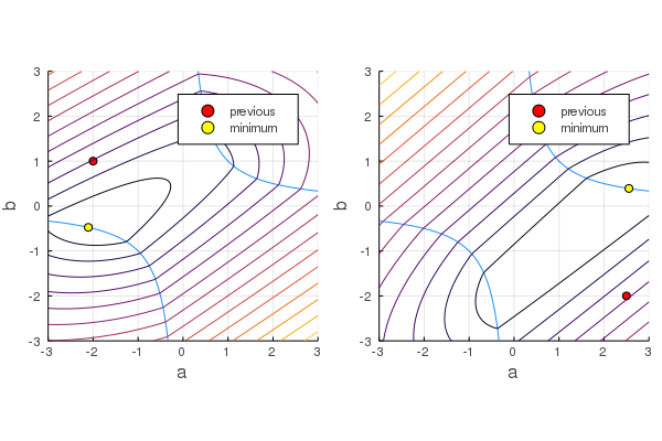
For these settings the values of $a$ and $b$ in the minimum point satisfy the bilinear equality constraint.

Citing the package and/or method

Citations are appreciated if you use this software for academic purposes.

The method:

@inproceedings{doelman2016sequential,
  title={Sequential convex relaxation for convex optimization with bilinear matrix equalities},
  author={Doelman, Reinier and Verhaegen, Michel},
  booktitle={2016 European Control Conference (ECC)},
  pages={1946--1951},
  year={2016},
  organization={IEEE}
}

The software:

@misc{SequentialConvexRelaxation,
  author={Reinier Doelman},
  title={SequentialConvexRelaxation.jl},
  howpublished={\url{https://github.com/rdoelman/SequentialConvexRelaxation.jl/}},
  year={2019}
}