Training neural networks with convex optimization

A basic neural network consist of interconnected layers with nodes. The nodes apply an activation function on a weighted combination of the outputs of the nodes of the previous layer. Given some data and corresponding measurement, an objective function relates predicted measurements (based on the current estimate of the weights) with the actual measurements. By far the most popular way to optimize (‘training’) the weights in a neural network, is to use gradient descent on this objective function. There are several reasons to go about training the weights this way, of which some are:

• the involved objective functions are nonlinear and non-convex,
• they are continuous and (sub)differentiable,
• the gradients can be computed efficiently and fast,
• the method can be applied to very large datasets.

Even though the objective function is non-convex, one might wonder whether there are convex optimization problems that yield the correct result, i.e. the best trained weights.

By analogy, think of least squares problems $\| y - Ax \| ^2$ with sparse vectors $x$. Even though cardinality constraints (constraints on the number of non-zero elements) make the estimation problem non-convex, using (convex) $\ell_1$ norm regularization (LASSO, (Tibshirani, 1996)) can under certain conditions result in the correct sparse solution (Candes, Romberg, & Tao, 2006).

The question is, can we do something similar for neural networks?

This way of looking at it is different from creating convex approximations of an objective function (Scardapane & Di Lorenzo, 2018). In fact, we apply the method in (Doelman & Verhaegen, 2016).

The rectified linear unit

A number of activation functions exist, but here we limit ourselves to rectified linear units, which apply the function $h = f(x) = \max(0,x)$ on an input $x$. This activation is widely used, so the choice is not very restricting.

The constraint $h = max(0, x)$ between variables $x$ and $h$ is equivalent to (Fischetti & Jo, 2017),

$$\begin{equation} \begin{aligned} x &= h - s \\ h &\geq 0 \\ s &\geq 0 \\ hs &= 0 \end{aligned} \end{equation}$$

The ReLU activation function can be rewritten into an equality constraint, two inequality constraints and a bilinear constraint. This is something we will exploit later on.

A basic neural network

For a neural network we denote the output of the $i$‘th node in the $j$‘th layer as $x^i_j$. The outputs of a single layer are grouped in a vector, denoted $x_j$. The weights for a node are collected in a vector $w$, which in turn can be collected row-by-row into a matrix $W$, such that the input for layer $j$ is formed according to $W_j x_{j-1} + b_j$, where $b_j$ is a vector of offsets. The function $f(x)$ is applied element-wise (indicated $f.(\cdot)$) to this vector, such that we have $x_j = f.( W_j x_{j-1} + b_j )$.

I constrict the analysis here to a neural network, with one hidden layer, that can exactly model the data. This means training the weights is a feasibility problem. The analysis for multiple layers is similar. The input vector is $x_0$ and output vector $y$ ($= x_2$). Let us further assume we collected $K$ input and output data points $x_{0,k},~ k = 1,\ldots,K$ and $y_k$. Collecting these in a matrix, we obtain $X_0 = \begin{bmatrix} x_{0,1} & \cdots & x_{0,k} \end{bmatrix}$ and $Y = \begin{bmatrix} y_{1} & \cdots & y_{k} \end{bmatrix}$. The complete equations for the neural network are therefore

$$\begin{equation} \begin{aligned} X_1 &= f.(W_1 X_0 + B_1), \\ Y &= f.(W_2 X_1 + B_2), \end{aligned} \end{equation}$$

where $B_1 = b_1 \otimes \mathbf{1}, ~ B_2 = b_2 \otimes \mathbf{1}$, $\mathbf{1}$ is a vector of all ones, and $\otimes$ denotes the Kronecker product. $X_1$ is defined similar to $X_0$.

Rewriting the expressions for the neural network

Next, we introduce $Z_1 = W_1 X_0 + B_1$ and $Z_2 = W_2 X_1 + B_2$. Then we have

$$\begin{equation} \begin{aligned} X_1 &= f.(Z_1), \\ Y &= f.(Z_2). \end{aligned} \end{equation}$$

The final thing we do, is using the relation in equation (1) to get rid of the function $f$. This results in the following set of equations, that are equivalent to (2):

$$\begin{equation} \begin{aligned} Z_1 &= X_1 - S_1, \\ 0 &= X_1 \odot S_1 \\ X_1 &\geq 0 \quad \text{(element-wise)}\\ S_1 &\geq 0 \quad \text{(element-wise)}\\ Z_2 &= Y - S_2 \\ 0 &= Y \odot S_2 \\ S_2 &\geq 0 \quad \text{(element-wise)} \\ Z_1 &= W_1 X_0 + B_1, \\ Z_2 &= W_2 X_1 + B_2 . \end{aligned} \end{equation}$$

The notation $\odot$ is used to express an element-wise product of the matrices.

What did all this rewriting accomplish? We got rid of all the functional expressions, and obtained a set of equations that can be split into two groups: one group contains the affine constraints and inequalities, and the other group contains all the bilinear equalities.

The affine constraints and inequalities:

$$\begin{equation} \begin{aligned} Z_1 &= X_1 - S_1, \\ X_1 &\geq 0 \quad \text{(element-wise)}\\ S_1 &\geq 0 \quad \text{(element-wise)}\\ Z_2 &= Y - S_2 \\ 0 &= Y \odot S_2 \\ S_2 &\geq 0 \quad \text{(element-wise)} \\ Z_1 &= W_1 X_0 + B_1. \\ \end{aligned} \end{equation}$$

The bilinear constraints:

$$\begin{equation} \begin{aligned} 0 &= X_1 \odot S_1 \\ Z_2 &= W_2 X_1 + B_2 . \end{aligned} \end{equation}$$

A rank-constrained reformulation for a neural network

The point of all this rewriting is to come to a group of bilinear constraints for which we can construct a convex heuristic. We can reformulate these bilinear constraints into (sets of) rank constraints, and for these rank constraint we can use the nuclear norm as a convex heuristic.

What we will use is the following substitution. We substitute constraints of the form $APB=C$, where $A, ~B,~ C$ are decision variables and $P$ is some matrix, with the rank constraint

$$\begin{equation*} \begin{aligned} \text{rank}~M(A,P,B,C,Q,R) &= \text{rank}~P \\ M(A,P,B,C,Q,R) &= \begin{bmatrix} C + APR + QPB + QPR & (A + Q)P \\ P(B + R) & P \end{bmatrix} \end{aligned} \end{equation*}$$

and where $Q$ and $R$ can be any matrix of appropriate size. These are not decision variables, these are parameters. The matrix $M$ is affine in $A,~B$ and $C$, a property we will use in just a bit.

We can now replace all the constraints in (6) with appropriate rank constraints:

$$\begin{equation} \begin{aligned} \text{rank}~M_1 &= \text{rank}~I_1, \\ \text{rank}~M_2 &= \text{rank}~I_2, \end{aligned} \end{equation}$$

where $I_1, I_2$ are identity matrices of appropriate size and where

$$\begin{equation*} \begin{aligned} M_1 & = M(\text{dv}(X_1),I,\text{dv}(S_1),0,\text{dv}(Q_1),\text{dv}(R_1)), \\ M_2 & = M(W_2,I,X_1,Z_2-B_2,Q_2,Q_1). \\ \end{aligned} \end{equation*}$$

and $\text{dv}(\cdot)$ is short for $\text{diag}(\text{vec}(\cdot))$ (a vectorized matrix on the diagonal of a new matrix, to rewrite element-wise multiplication into a matrix form).

Finding a $W_1, W_2, X_1, B_1, B_2$ that satisfy equation (2) is equivalent to finding variables $W_1, W_2, X_1, B_1, B_2$ and $Z_1, Z_2, S_1, S_2$ that satisfy the constraints

$$\begin{equation*} \begin{aligned} Z_1 &= X_1 - S_1, \\ X_1 &\geq 0 \quad \text{(element-wise)}\\ S_1 &\geq 0 \quad \text{(element-wise)}\\ Z_2 &= Y - S_2 \\ 0 &= Y \odot S_2 \\ S_2 &\geq 0 \quad \text{(element-wise)} \\ Z_1 &= W_1 X_0 + B_1. \\ \end{aligned} \end{equation*}$$

and

$$\begin{equation*} \begin{aligned} \text{rank}~M_1 &= \text{rank}~I_1, \\ \text{rank}~M_2 &= \text{rank}~I_2, \end{aligned} \end{equation*}$$

A convex heuristic

For rank constraints, the nuclear norm is a convex heuristic, the same ways as for cardinality constraint the $\ell_1$ norm is a heuristic. The convex heuristic for neural networks with ReLU activation functions is the convex optimization problem

$$\begin{equation} \begin{aligned} &\text{minimize} && \left\|M_1\right\|_* + \lambda\left\|M_2\right\|_* \\ & \text{subject to} && Z_1 = X_1 - S_1, \\ & && X_1 \geq 0 \quad \text{(element-wise)}\\ & && S_1 \geq 0 \quad \text{(element-wise)}\\ & && Z_2 = Y - S_2 \\ & && 0 = Y \odot S_2 \\ & && S_2 \geq 0 \quad \text{(element-wise)} \\ & && Z_1 = W_1 X_0 + B_1. \end{aligned} \end{equation}$$

where we introduced the weighting parameter $\lambda$ and $\left\| \cdot \right\|_*$ denotes the nuclear norm of a matrix, i.e. the sum of its singular values. This convex problem can be easily programmed using for example Convex.jl and solved with a compatible SDP solver.

Parameter settings

Apart from $\lambda$, we are left with choosing the parameters $Q_1,~Q_2$ and $R_1$. These are matrices with the same size as $X_1,W_2$ and $S_1$ respectively. There are some possibilities for choosing them:

1. set them to 0,
2. set them to a matrix with randomly generated elements,
3. set them to the true values of $-X_1,-W_2$ and $-S_1$ (of the neural network that generated $Y$ based on $X_0$),
4. set them to a value related to the optimal parameters of a previously solved problem to obtain an iterative method.

With the values in option (3), the optimal solution to the convex problem in (8), consists again of the true values for $X_1,X_2,W_2$ and $S_1$, which can be verified by substituting the values. That means that there is at least one convex optimization problem whose solution gives the optimally trained weights in the neural network.

Numerical results

I generated a neural network with randomly chosen weights and 30 inputs and outputs. There are 3 input nodes, 3 hidden nodes in 1 layer, and two output nodes:

I implemented the procedure of item number 4 (updating the parameters with the negative values of the optimal variables each iteration), i.e.

1. Initialize $Q_1,Q_2,R_1$
2. Solve (8)
3. Set $Q_1 = -X_1^*,~Q_2 = -W_1^*$ and $R_1 = -S_1^*$.
4. Go to 2

In step 3, the superscript ${}^*$ denotes the optimal value of the parameter.

Here the initial parameters are perturbed optimal values, and in thirty iterations we found parameter settings that produce the exact measurements. This produces the following converging bilinear constraint violations:

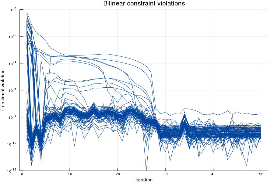
With all the constraint violations converged to the numerical precision of the solver, we have all constraints in (4) satisfied, which means that the produced parameters exactly model the data.

The resulting trained weights turned out to be different from the true parameters, but generated the exact same outputs (because they are a feasible solution of (5) and (6)).

I also tried starting with random starting values, and obtained the results below.

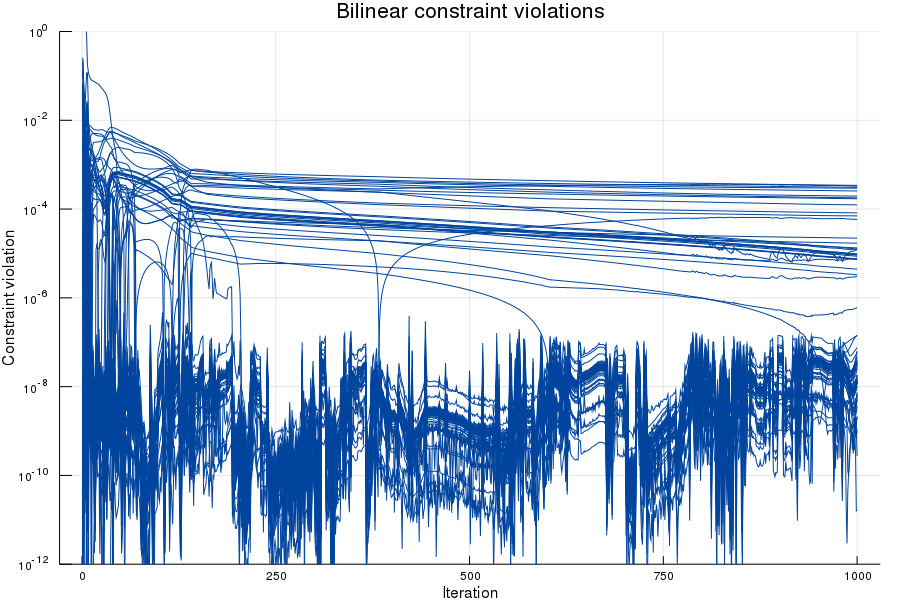
Now, the procedure did not produce variables that exactly fit all the bilinear constraints (although the constraint violations seem to very slowly decrease). But, after checking, the weights that are estimated generate the correct outputs (with a normed difference in the order of $10^{-8}$) within 50 iterations.

Initialization of the iterative procedure with $Q_1,Q_2,R_1$ equal to 0 gave a similar results.

Conclusion

So what can we conclude from this analysis?

First, that the training of neural network with ReLU activation functions can be rewritten into rank constrained optimization problems.

Second, that there is an infinite number of differently parameterized convex optimization problems that are a convex heuristic for training these neural networks.

Third, there are convex optimization problems whose optimal parameter values give a perfectly trained neural network.

Fourth, if we were unlucky enough to choose the wrong initial parameter values, we can try a new heuristic convex optimization problem based on the result of the previous problem. For the example case, this iteration produced a perfectly trained neural network.

What are the downsides of this approach?

First and foremost, there is no guarantee to find the optimal values. Maybe they can act as a good initialization for a gradient descent procedure, but how well this works is something that still has to be investigated.

Secondly, the method is very computationally expensive. Using the nuclear norm is an computationally expensive operator and there is no guarantee that the correct solution is found in just a few iterations.

Some future things to figure out are (computing time) scalability, convergence guarantees and parameter update strategies.

Bibliography

1. Tibshirani, R. (1996). Regression shrinkage and selection via the lasso. Journal of the Royal Statistical Society: Series B (Methodological), 58(1), 267–288.
2. Candes, E. J., Romberg, J. K., & Tao, T. (2006). Stable signal recovery from incomplete and inaccurate measurements. Communications on Pure and Applied Mathematics: A Journal Issued by the Courant Institute of Mathematical Sciences, 59(8), 1207–1223.
3. Scardapane, S., & Di Lorenzo, P. (2018). Stochastic training of neural networks via successive convex approximations. IEEE Transactions on Neural Networks and Learning Systems, (99), 1–10.
4. Doelman, R., & Verhaegen, M. (2016). Sequential convex relaxation for convex optimization with bilinear matrix equalities. In 2016 European Control Conference (ECC) (pp. 1946–1951). IEEE.
5. Fischetti, M., & Jo, J. (2017). Deep neural networks as 0-1 mixed integer linear programs: A feasibility study. ArXiv Preprint ArXiv:1712.06174.