Tensorflow is hugely popular as deep learning software and it allows for both high-level and low-level customization. In principle, its purpose is to define a neural network, and optimize/train the weights in each layer through the method of gradient descent.
There are other optimization problems that are not solved through a gradient descent method, like combinatorial optimization problems. One of the most common combinatorial problems are mixed-integer linear programming (MILP) problems. The problems have linear objective functions and affine (in)equality constraints on variables that are either continuous, or integer-valued.
In this post, we will analyze a programming problem where all values should take either the value 0 or the value 1, called binary programming problems. As an example problem we will try to solve a sudoku using Tensorflow’s gradient-based optimization functionality.
The code is available in a Jupyter notebook.
The sudoku
A sudoku can be seen an optimization problem with 9x9x9 = 729 binary variables . Each square (i,j) in a sudoku has 9 variables associated to it, that each indicate if this square should hold the number .
Given a number of hints (pre-filled squares), the rules of sudoku then specify that:
- each column has each number 1 to 9 once and only once
- each row has each number 1 to 9 once and only once
- each of the 9 3x3 blocks has each number 1 to 9 once and only once.
These constraints can be reformulated to constraints on the values of . For example, the fact that only one number is filled in can be described as for all squares (i,j). The rule that each column contains the numbers 1 to 9 can be described as for all columns j and numbers k. The other rules work similarly.
The Sudoku layer
Tensorflow’s documentation has a nice example on how to define a custom layer, so let’s define the Sudoku layer.
A sudoku layer receives as input the sudoku hints and as output produces some measure (loss) of how well its internal state fits with the hints and how well it respects the rules of the puzzle.
Its internal state consists of a trainable 9x9x9 tensor of continuous variables x (the ‘weights’), and an untrainable 9x9x9 parameter tensor w. We’ll initialize these as follows:
class Sudoku(layers.Layer):

    def __init__(self):
        super(Sudoku, self).__init__()
        x_init = tf.random.uniform([9,9,9], minval=0, maxval=0.5, seed=123)
        self.x = tf.Variable(initial_value=x_init,
                             trainable=True)
        w_init = 1.0-2.0*self.x
        self.w = tf.Variable(initial_value=w_init,
                             trainable=False)
Now we need to figure out a couple of things:
- how to penalize violations of the rules of the puzzle,
- how to penalize the variable x such that it ends up as 0 or 1.
The loss functions
Tensorflow allows one to assign losses to a layer and extract them at a later point. This makes it more convenient to forget about the layer output (just set it to 0 and use the layer losses).
There are three types of constraint we will try to enforce:
- equality constraints (like )
- interval constraints (like a bound )
- integrality constraints ( is 0 or 1)
To enforce the first type, we add something like to our loss function (i.e. we use a barrier function as a loss). This will penalize the inequality with an absolute value-based loss.
For Tensorflow, this looks as follows.
# Penalties for violations of the rules of sudoku
cols = tf.reduce_sum(self.x, axis=0) - 1.
constraint_loss = tf.reduce_sum(tf.math.abs(cols))

rows = tf.reduce_sum(self.x, axis=1) - 1.
constraint_loss += tf.reduce_sum(tf.math.abs(rows))

blocks = tf.reshape(self.x, [3, 3, 3, 3, 9])
blocks = tf.reduce_sum(blocks, axis=[1, 3]) - 1.
constraint_loss += tf.reduce_sum(tf.math.abs(blocks))

singles = tf.reduce_sum(self.x, axis=2) - 1.
constraint_loss += tf.reduce_sum(tf.math.abs(singles))

assignment = tf.math.multiply(self.x, hint_select) - hint_offset
constraint_loss += tf.reduce_sum(tf.math.abs(assignment))

G = 20. # tuning parameter
self.add_loss(G * constraint_loss)
The variables hint_select and hint_offset are the hints of the sudoku written in tensor format. Tensorflow just isn’t a fan of list comprehension…
The variable G is a tuning parameter that will allow us to weigh the different types of losses against each other.
For the interval constraint we use the rectified linear unit:
# Penalty to keep x between 0 and 1
interval = tf.nn.relu(self.x - 1.) + tf.nn.relu(-self.x)

self.add_loss(G * tf.reduce_sum(interval))
This loss is 0 if the elements of x are all between 0 and 1, so again a barrier function as a loss.
So, finally, how do we obtain values of x being 0 or 1?
We’ll try to do that using the following loss, that involves the parameter w:
# Penalty to steer x to 0 or 1
to_01 = tf.math.abs(4.*tf.math.multiply(self.w,self.x) +
    tf.math.multiply(self.w,self.w) + 1. - 2.*self.w)

self.add_loss(tf.reduce_sum(to_01))
In proper notation, this is the loss .
This loss is a heuristic convex method to stimulate x in the direction of 0 or 1, depending on w.
If w[i,j,k] is between -1 and 0, it stimulates x[i,j,k] towards 0, if it is between 0 and 1 it stimulates x[i,j,k] towards 1. Just don’t set it to 0.
Once we have optimized all the losses over x, we change w to 1-2x and minimize the loss again: we iteratively try to push the elements of x to 0 or 1.
The upside of this is that in each iteration the subproblem is convex and differentiable. And once we are done, we can check if all the constraints are satisfied. However, the method is still heuristic, and we are not guaranteed that we will always find a correct solution (and in more general problems, the best solution). That is where actual MILP solvers (or sudoku solvers) come in.
Solving the sudoku
We defined a Sudoku layer, and this layer has losses associated with it.
To train this layer, we repeatedly present the same sudoku hints over and over to the input of this layer as the problem ‘data’, and use gradient descent to minimize the loss function.
# Instantiate an optimizer.
optimizer = tf.keras.optimizers.Adam()

# Iterate over the batches of a dataset.
s = Sudoku()
s(hint_select, hint_offset) # initialize the losses
for i in range(10):
    print("Epoch", i)

    for j in range(4000):
        with tf.GradientTape() as tape:
            # the 'data' here is just the same sudoku hints
            # in tensor form over and over
            s(hint_select, hint_offset)

            loss_value = sum(s.losses)

            grads = tape.gradient(loss_value, s.trainable_weights)
            optimizer.apply_gradients(zip(grads, s.trainable_weights))

    s.w = 1.0-2.0*s.x
Each inner iteration consists of 4000 gradient descent steps, which gets us close enough to every iteration’s minimum.
We then switch out w for a new value, and we repeat this 10 times or so.
If the values of x have converged to the correct values, you have solved a single sudoku.
To be clear, you now do not have a network that computes the answers to any sudoku presented to it by a single forward pass.
Example
You can find the full sudoku layer and this example in this Jupyter notebook.
The convergence plot of the tensor x looks something like this:
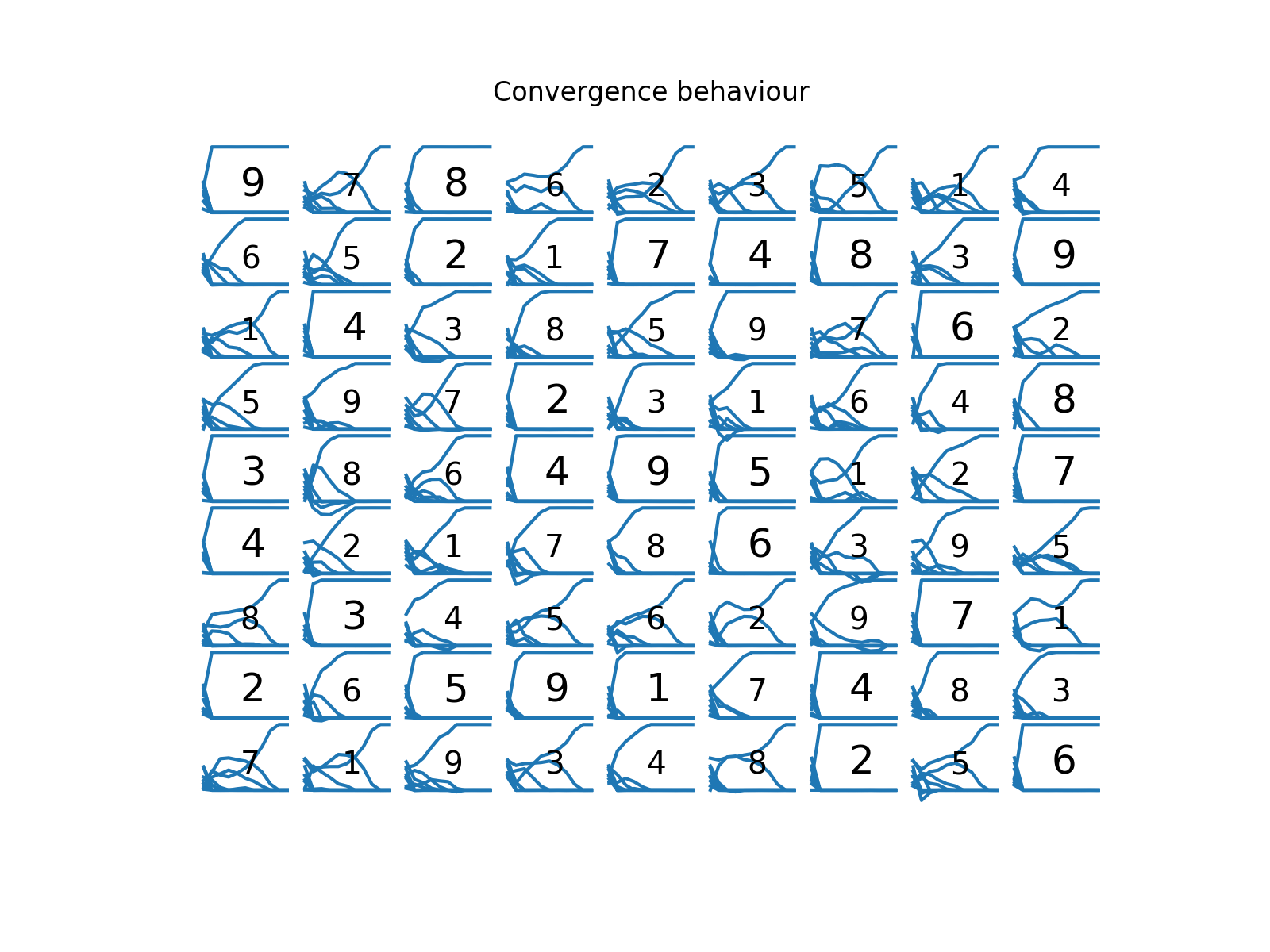
Each square (i,j) has its hint plotted (larger font) or the computed solution (smaller font).
Below that, there are the 9 trajectories of the elements in x[i,j,:].
We can see that all the elements of x slowly but surely converged to 0 or 1.
The final loss function itself is 0 (when we round the values of x at the end), so no constraints are violated and we can conclude that we found the correct solution to this sudoku.
Conclusions
In this post, I showed how the gradient-based optimization capabilities of Tensorflow can be used for something different: solving mixed-integer linear programming problems. I made this concrete by introducing a sudoku layer for solving a specific type of MILP problem: a sudoku. The method however is more general, but requires, just like here, some tuning and a good (‘lucky’) initialization.
Afterword
Using the Julia programming language and the Flux machine learning library.
To test the viability of solving a sudoku with gradient descent, I’ve programmed this using the combination of Python and Tensorflow. I also did this using the combination of the Julia programming language and the Flux machine learning package. The reason is that with Flux the sudoku constraints are easily described with list comprehensions. I’ve personally found it much more productive.
Here’s the sudoku layer definition:
mutable struct SudokuLayer
    x
    w
end
SudokuLayer(x) = SudokuLayer(x, 1f0 .- 2f0*data(x))
And here’s the computation of the loss functions:
function (s::SudokuLayer)(hints)

    # rules of the sudoku puzzle
    cols = [reduce(+, s.x[:,j,k]) - 1f0 for j = 1:9, k = 1:9]
    rows = [reduce(+, s.x[i,:,k])  - 1f0 for i = 1:9, k = 1:9]
    blocks = [reduce(+, s.x[i:i+2,j:j+2,k])  - 1f0 for i in (1,4,7), j in (1,4,7), k = 1:9]
    singles = [reduce(+, s.x[i,j,:])  - 1f0 for i = 1:9, j = 1:9]

    # hints
    assignment_1 = [s.x[i,j,k] - 1f0 for i in 1:9, j in 1:9, k in 1:9 if hints[i,j] == k]
    assignment_0 = [s.x[i,j,k] for i in 1:9, j in 1:9, k in 1:9 if all(hints[i,j] .!= (k,0))]

    # interval constraint
    interval = map(x->relu(x-1)+relu(-x),s.x) # x in [0,1]

    to_0_or_1(x,w) = abs(1f0 + 4f0*w*x - 2f0*w + w^2)
    to_0(x) = abs(x)
    constraints = mapreduce(
        v -> vcat(v[:]),
        vcat,
        [
         cols,
         rows,
         blocks,
         singles,
         assignment_0,
         assignment_1,
        ],
    )
    return (map(to_0, constraints), interval, map(to_0_or_1, s.x, s.w))
end
Acknowledgements
My thanks go to Wiegert Krijgsman, who pointed out to me that the use of the nuclear norm operator as a convex heuristic for 0-1 constraints has a more elegant formulation using the absolute value function.