Training a classifier on 1 billion data points in under 3.5 minutes on a laptop.

Introduction

One of the key rules of applied optimization research or data science is that there’s always someone with a problem with more data to process than you. So let’s talk about training classifiers on really large datasets. What I’ll discuss is: how can you train classifiers when the amount of data you have becomes too large for standard techniques, such as ScikitLearn’s LinearRegression, to handle?

Key ingredients

Some of the key concepts for training a classifier on a really large dataset are the following:

• Look at data once (if possible);
• Be careful with the amount of memory your method uses;
• Put priority on algorithms that can be distributed across devices and servers.

How can one accomplish this practically? Well, in the same order as the list above:

• use a stochastic gradient descent method that updates the classifier using a single data point or a batch of points, and simple pass the data through
• Up front, decide to use a training algorithm that can be implemented using a fixed amount of memory. If it’s fixed, you wont run into trouble.
• Some classifiers can be merged to produce a classifier that works on data that either one has seen. Choose one of those.

So, what software? I used

• Julia
• Julia’s parallel computing functionality
• The package OnlineStats.jl

There’s one more key ingredient. The OnlineStats.jl package has ready made implementations available for normal linear regression with both constant memory and the ability to merge classifiers. However, a dataset with two classes does not have to be linearly separable. Therefore, we use a random nonlinear transformation, a random mapping to a higher dimension called a Random Fourier (or Feature) Expansion (RFE). This is a transformation of the form

where $\Omega$ is a random matrix, Ω = σ*randn(D,n) (D is the number of higher dimensions, n the number of features, and σ is a tuning parameter), and $b$ a vector, b = 2π * rand(n). An explanation of where this comes from you can find here. This mapping allows us to estimate a simple linear model in the higher dimension, which translates to a nonlinear model in the lower dimension. Furthermore, we technically do not need anyone to tell us the real input $x$, only $f(x)$. And since the $\cos$ operation is not invertible, it’s pretty hard if not impossible, to figure out what the original $x$ was.

Implementation

The implementation is relatively simple thanks to the building blocks that OnlineStats.jl and Julia provide.

using Distributed
@everywhere using OnlineStats.jl
using LinearAlgebra
using Random
Random.seed!(1)

σ0 = 0.3 # noise level class 0
σ1 = 0.1 # noise level class 1
# Generate a sample that with probability r belongs to class 1, 1-r to class 0.
@everywhere function new_sample(r) # ScikitLearn's 'half moon' dataset
    if rand() < r
        return π*rand() |> t -> ([cos(t) + $σ1*randn(), sin(t) + $σ1*randn()],1)
    else
        return π*rand() |> t -> ([1.0 - cos(t) + $σ0*randn(), 1.0 - sin(t) - 0.5 + $σ0*randn()],0)
    end
end

# Training a classifier
# Map the features nonlinearly to a higher dimension
# feature transform function u((x,y)) -> (f(x),y)
D, n, Ω, b = 9, 2, 0.6*randn(D,n), 2π*rand(D)
@everywhere u(z) = (cos.($Ω*z[1] + $b), z[2])

N = 1E9
p = nprocs()
h = @timed begin
    lr = @distributed merge for i in 1:p
        o = FTSeries( LinReg(D), transform = u )
        fit!(o, (new_sample(0.5) for i in 1:round(Int,N/p)+1))
    end
end
println("Trained on $(nobs(lr)) samples in $(h[2]) seconds.")

The function that maps an input to a scalar between 0 and 1 is:

c = coef(lr.stats[1],1E-6)
sigmoid(x) = 1. / (1. + exp(-(x - 0.5)))
df(x) = dot(c, cos.(Ω*x + b)) |> sigmoid

What does this code do? OnlineStats.jl takes care of the training by streaming new samples to the computed classifiers and updating them. Then it merges the result from p independent processes (/classifiers), that are each trained on 1/p of the samples.

Result

Running the code above on my laptop results in the following output:

Trained on 1000000008 samples in 209.822495601 seconds.

That’s over a billion samples in three and a half minutes on my laptop’s CPU.

The resulting decision function looks as follows:

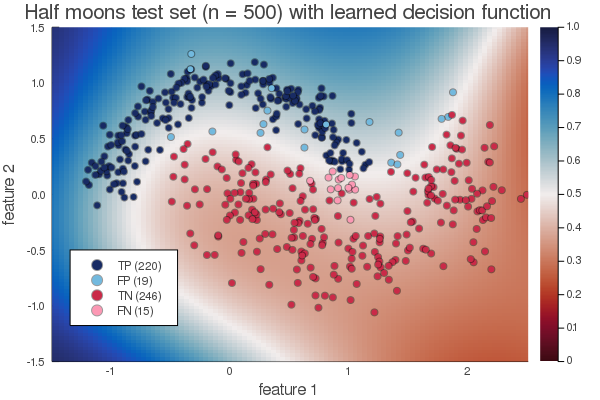
I’ve added 500 points from the different classes to this image to make clear how the data is distributed.

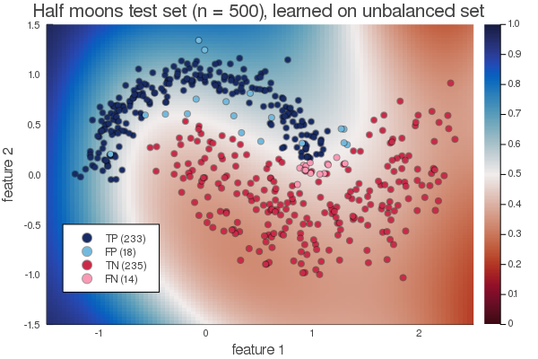
Another feature of OnlineStats.jl is that it’s easy to compensate for class imbalances. That is, if one class is much more prevalent than the other one. We can simply penalize an error in this minority class more when we update the classifier with a new sample from this class. Here’s a result with a ratio of the data points of 1:100.000 between the classes, again trained on a billion data points:

Quick comparison with ScikitLearn

The ScikitLearn python package’s LinearRegression function uses LAPACK under the hood. It works by presenting the entire dataset at once to LAPACK. That requires a lot of memory, and my laptop maxed out at about 1 million samples. However, it’s no problem for OnlineStats.jl since we can stream new data to the solver and immediately forget that data point; we’re looking at it once and only once. Below you can see the difference in training time:

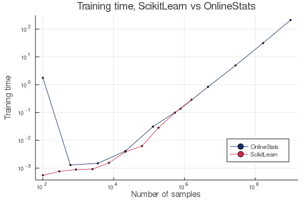
The first data point for OnlineStats.jl with 100 samples I believe is an artefact of Julia’s compilation time and should be ignored.

Conclusion

The code above has 31 lines. The problem-solving-part only needs 13. If you’re inundated with data your first reaction doesn’t necessarily need to be that one of bigger computing power and memory. It should be better tools. Only after using better tools, the question should be how much computing power you really need. Fortunately, that doesn’t need to imply that these tools need to be more complex.